Simulating Correlated Likert Scale Data

Simulating Correlated Likert-Scale Data In R: 3 Simple Steps

Let us simulate some data!

Imagine you have sent out a questionnaire measuring a Construct using six items on a 7-point likert-scale.

You’re impatiently waiting for the responses and you want to start creating your data analysis code so you only have to insert the gathered data once it arrives. To make this process smooth, you want to have some realistic simulation of your actual data.

In the following lines of code, I will show you how to simulate the ideal scenario of intercorrelated Likert-Scale answers that measure one underlying factor (construct).

Loading the libraries

Let’s start by loading the libraries.

library(polycor) # for polychoric correlations
library(psych) # for scree plots
library(tidyverse)
library(faux) # for the function rnorm_pre
library(truncnorm) # for the function rtruncnorm

Creating simulation data

Step 1: Create a single item

The package truncnorm provides a function to sample data from a normal distribution, but with boundaries (“truncated”)! This is just what you want, as your data will be on a 7-point scale. a and b will be the truncation limits. As I want to center my values around a mean of 0, I will use -3 and 3. To get plausible likert-scale integers, I just use the round function. As it’s sampled data, it doesn’t really matter if the mean is not exactly zero.

##### SIMULATE DATA ######
# simulate NPI_1
NPI_1 <- round(rtruncnorm(n = 500, 
                    mean = 0, 
                    sd = 1,
                    a = -3,
                    b = 3))
head(NPI_1)

## [1]  0 -1  1  2 -1  0

mean(NPI_1)

## [1] -0.028

Step 2: Get its correlated cousins

Now we can use the rnorm_pre function from the faux package to simulate data that is correlated to our first item. For this, we set the same parameters (mu is the mean) as our original item and set the correlations (r) to medium to strong correlations. Again, we use the round function to make it a likert-scale data. In the end, we can combine these data in a data.frame.

# get correlated NPI_2:
NPI_2 <- round(rnorm_pre(NPI_1, mu = 0, sd = 1, r = 0.7))
NPI_3 <- round(rnorm_pre(NPI_1, mu = 0, sd = 1, r = 0.6))
NPI_4 <- round(rnorm_pre(NPI_1, mu = 0, sd = 1, r = 0.7))
NPI_5 <- round(rnorm_pre(NPI_1, mu = 0, sd = 1, r = 0.8))
NPI_6 <- round(rnorm_pre(NPI_1, mu = 0, sd = 1, r = 0.75))


NPI <- tibble(NPI_1, NPI_2, NPI_3, NPI_4, NPI_5, NPI_6)
head(NPI)

## # A tibble: 6 x 6
##   NPI_1 NPI_2 NPI_3 NPI_4 NPI_5 NPI_6
##   <dbl> <dbl> <dbl> <dbl> <dbl> <dbl>
## 1     0    -1     1     0     0     1
## 2    -1     0    -2    -1    -1     0
## 3     1     0     0     1     1     1
## 4     2     1     1     1     2     3
## 5    -1    -2    -1     1     0    -1
## 6     0     1     0     0     1     1

Step 3: Check the assumptions

Great! Now that we have our simulated data from six items, we want to check whether they all load on one underlying latent factor. For this, we can use polychoric correlations, but Pearson correlations might be applicable too, see the book Modern Psychometrics in R. The hetcor function from the polycor package calculates

“A detailed study of this phenomenon within the context of structural equation models can be found in Rhemtulla et al. (2012). The authors suggest that in the area of 6, 7, or more categories, differences between Pearson and polychoric become negligible.”

See also here to learn how polychoric correlations work.

cormat <- hetcor(NPI) # calculate correlation matrix
eigen_values <- eigen(cormat)

scree(cormat$correlations, factors = FALSE) # nice

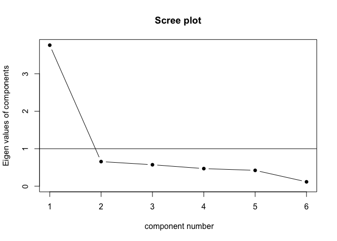
Cool! We actually seem to have one underlying component, as the “elbow” of the scree plot is behind the first component - see here for an explanation of scree plots.

Now let’s check the internal consistency using a custom-made cronbach’s alpha function:

# check internal consistency (cronbach's alpha):
cronbach.alpha <- function(data){
  k <- ncol(data)
  vcmat <- cov(data, use = "pairwise")
  sigma2_Xi <- sum(diag(vcmat))
  sigma2_X <- sum(vcmat)
  alpha <- k/(k-1)*(1-sigma2_Xi/sigma2_X)
  return(alpha)
}
cronbach.alpha(NPI) 

## [1] 0.8777856

We seem to have a good internal consistency of the used scale! Horray!

You can now start using the data for your investigations, as if you’re using real data!